Data generation
We can simulate from a branching process to form a data set of transmission trees or clusters (if we remove infector information from the transmission trees). We simulate \(K\) branching processes where the primary infector in each tree is the root of each transmission tree and the probability of infection of another individual is where \(\bf{X}\) is a covariate matrix and \(\beta\) is a vector of coefficients, \[ p_i = logit^{-1} (\bf{X}_i\bf{\beta}). \] Then the number of new infectious individuals infected by individual \(i\) is \[ N_i \sim Geometric(p_i). \]
To form a branching process, we begin with an initial infector who is the root node who we index as (1,1). We then draw \(N_{(1,1)} \sim Geometric(p_{(1,1)})\), the number of infections produced by individual (1,1). These infections are part of generation 2 and so will be given indices \((2, 1), \dots, (2, N_{1,1})\).
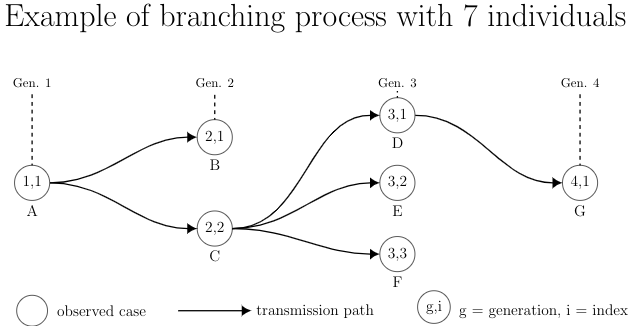
The infection proceeds by marching down the generations. We first draw \(N_{(2,1)}\) (if individual (2,1) exists) and give these new infections indices \((3, 1), \dots, (3, N_{(2,1)})\). We then draw \(N_{(2,2)}\) and assign them indices \((3, N_{(2,1)} + 1), \dots, (3, \sum_{i=1}^{2}N_{2,i})\). We repeat this process until all infections in generation 3 are achieved. We then repeat the process beginning in generation 4. This infection process is repeated until it naturally terminates (or too a maximum number of infections are drawn). This process is illustrated in the below figure.

Then the data for a single transmission tree is a matrix of size \(n\) where each row is the form \((label, g, i, \inf g, \inf i)\), where label denotes the individual and refers to her covariates, \((g,i)\) is the indexing of individual \(A\) and \((\inf g, \inf i)\) is the infector ID or is denoted by \(\emptyset\) to show that the infection originated from outside the cluster. For example, the above transmission tree \(T\) becomes \[ T = \left ( \begin{array}{ccccc} A& 1& 1& \emptyset& \emptyset&\\ B& 2& 1& 1& 1\\ C& 2& 2& 1& 1\\ D& 3& 1& 2& 2\\ E& 3& 2& 2& 2\\ F& 3& 3& 2& 2\\ G& 3& 4& 3& 1 \end{array}\right ), \] where \(\emptyset\) means we assume the infection originates from the outside.
Computing the likelihood of a tree \(T\)
Because we know the transmission tree, we know \(N_{g,i}\), the number of infections transmitted by indivdual \((g,i)\). In terms of our above matrix \(T\), this is found by counting the number of infector generation, index pairs that equals the individual’s own generation, index pair. For example, in the above, \(N_{(1,1)} = 2, N_{(2,1)} = 0, N_{(2,2)} = 3, N_{(3,1)} = 1, N_{(3,2)} = 0, N_{(3,3)} = 0, N_{(4,1)} = 0\). The likelihood is then the product of independent geometric random variables with different probabilities of success \(p_i\), \[ L(T) = \prod_{j=1}^n (1-p_j)p_j^{N_j}, \] where we use \(j\) as the label of the individual.
Computing the likelihood of an observed cluster \(C\)
In practice, we do not see the transmission tree \(T\) but are instead working with a missing data problem. We observe a cluster \(C\) of individuals, which is a collection of individuals along with their covariates. With respect to the above example matrix of \(T\), we would say \(C\) is a subset of \(T\), specifically \(C = (A, B, C, D, E, F, G)^T\). We say that the size of \(C\) is the number of individuals, \(|C| = n\) or 7 in the above example. We neither know the generation-index pairs nor the infector IDs of the individuals.
We thus compute the total likelihood \(\mathcal{L}(C)\) of a cluster, which is equal to the sum of the likelihood across the set of all permissible transmission trees, \(\mathcal{T}_C\), \[ \mathcal{L}(C) = \sum_{T \in \mathcal{T}_C} L(T). \]
Permissible Transmission Trees
We say a transmission tree \(T \in \mathcal{T}_C\) is permissible if it is a possible outcome of our data generation process. More specifcially, a transmission tree \(T\) is permissible if it satifies the following criteria,
- \(T\) has \(|C| = n\) nodes.
- The \(n\) individuals are placed into \(g\) successive generations where \(g\) is between 1 and \(n\), inclusive.
- The number of individuals in each generation is a \(g\)-tuple \((n_1, \dots, n_g)\) such that \(\sum_{j=1}^{g}{n_j} = n\) and \(n_j > 0\) for \(j =1, \dots, g\).
- There is exactly one root node so \(n_1 =1\).
- Each individual is indexed by \((h,i)\) which is the generation-index pair, where the index is the order of appearance within the generation, ranging between \(i=1, 2, \dots, n_h\).
- For \(g >1\), an individual \((g,i)\) has exactly one infector from generation \(g-1\). For \(g=1\), the infector is denoted by \((\emptyset, \emptyset)\).
- Each individual is assigned a label.
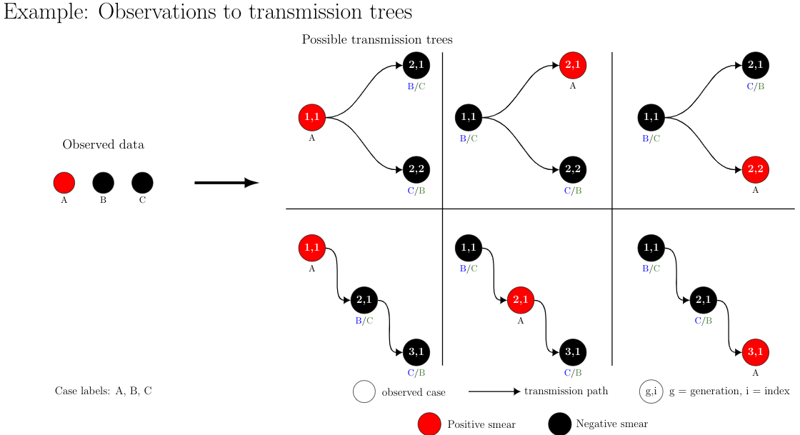
Ex. \(C = (A,B,C)\) where individual \(A\) has \(X_A = 1\) and individuals \(B\) and \(C\) have \(X_B = X_C = 0\)
The below figures shows the different trees in \(\mathcal{T}_C\) where \(|C| = 3\). The size of \(\mathcal{T}_C\) is \(|\mathcal{T}_C| = 12\) if we consider individuals \(A\), \(B\), and \(C\) to be distinguishable from one another. If we say individuals \(B\) and \(C\) are indistinguishable from one another because they have the same value of \(X_i=0\), then there are only 6 unique transmission trees.
Obtaining the maximum likelihood estimate (MLE).
For observed independent clusters \(C_1, \dots, C_M\), we would like to find the maximum likelihood estimate (MLE) of \(\beta\) \[ \hat{\beta}^{(MLE)} = \arg \max_\beta \prod_{m=1}^M\mathcal{L}(C_m). \]
However, if \(|C_m| > 15\), this is infeasible because the space of \(| \mathcal{T}_C|\) is too large. We can instead sample permissible transmission trees to solve an equivalent problem, maximizing the average likelihood.
Let the average likelihood of a single cluster \(C\) be given by \[ \bar{\mathcal{L}}(C) = \frac{\mathcal{L}(C)}{|\mathcal{T}_C|} \] and note that since \(|\mathcal{T}_C|\) is not dependent on \(\beta\) then the MLE is the same for both \(\mathcal{L}(C)\) and \(\bar{\mathcal{L}}(C)\), \[ \hat{\beta}^{(MLE)} = \arg \max_\beta \prod_{m=1}^M\mathcal{L}(C_m)\\ = \arg \max_\beta \prod_{m=1}^M\frac{1}{|\mathcal{T}_m|}\mathcal{L}(C_m)\\ = \arg \max_\beta \prod_{m=1}^M\bar{\mathcal{L}}(C_m). \]
We approximate average likelihood for each cluster through Monte Carlo (MC) sampling. For a given cluster \(C\), we sample \(K\) MC trees \(T_1, \dots, T_K \in \mathcal{T}_C\)and form estimates \[ \hat{\mathcal{L}}_K(C): = \frac{1}{K} \sum_{i=1}^KL(T_i) \overset{a.s.}{\to} \bar{\mathcal{L}}(C). \]
We then form our estimate \(\hat{\beta}^{(MC)}\) from Monte Carlo (MC) samples from \(\mathcal{T}_C\), \[ \hat{\beta}^{(MC)} = \arg \max_\beta \prod_{m=1}^M\hat{\mathcal{L}}_K(Cm). \]
The result is that (hopefully) \(\hat{\beta}^{(MC)} \approx \hat{\beta}^{(MLE)}\) if \(K\) is large. However, the limits of branching processes are sometimes found to be ‘non-standard’, meaning non-normal. As such, we demonstrate the usefulness of our methods through simulations.