aggregate SIR path visuals from agent data

aggregate SIR path visuals from agent data

geom_aggregate(
  mapping = NULL,
  data = NULL,
  stat = StatSirAggregate,
  position = "identity",
  ...,
  na.rm = FALSE,
  show.legend = NA,
  inherit.aes = TRUE
)

stat_aggregate(
  mapping = NULL,
  data = NULL,
  geom = "path",
  position = "identity",
  na.rm = FALSE,
  show.legend = NA,
  inherit.aes = TRUE,
  ...
)

Arguments

mapping	Set of aesthetic mappings created by aes() or aes_(). If specified and inherit.aes = TRUE (the default), it is combined with the default mapping at the top level of the plot. You must supply mapping if there is no plot mapping.
data	The data to be displayed in this layer. There are three options: If NULL, the default, the data is inherited from the plot data as specified in the call to ggplot(). A data.frame, will override the plot data. A function will be called with a single argument, the plot data. The return value must be a data.frame, and will be used as the layer data. A function can be created from a formula (e.g. ~ head(.x, 10)).
stat	Override the default connection between geom_aggregate() and StatSirAggregate stat to process raw data
position	Position adjustment, either as a string, or the result of a call to a position adjustment function
...	Other arguments passed on to layer(). These are often aesthetics, used to set an aesthetic to a fixed value, like colour = "red" or size = 3. They may also be parameters to the paired geom/stat.
na.rm	when using the default Stat or Geom this parameter doesn't matter as NAs are seen as encoders of information and NOT removed. See details for more on this. If not using either of these (which means this geom/stat doesn't need to be used), then if FALSE, the default, missing values are removed with a warning. If TRUE, missing values are silently removed.
show.legend	logical. Should this layer be included in the legends? NA, the default, includes if any aesthetics are mapped. FALSE never includes, and TRUE always includes. It can also be a named logical vector to finely select the aesthetics to display.
inherit.aes	If FALSE, overrides the default aesthetics, rather than combining with them. This is most useful for helper functions that define both data and aesthetics and shouldn't inherit behaviour from the
geom	Override the default connection between stat_aggregate() and geom_path().

Details

This visual leverage the function agents_to_aggregate underneath. This function converts individual agents' information on when the agent transitions between 3 different states (ordered), to create a temporal tally/aggregation of how many agents are in what state at each integer time point. In this visualization tool, the user provides y and z to present the agent enters the second and third state (respectively).

As mentioned in parameter details, agents_to_aggregate encodes NA to capture information, and as such, the default

Aesthetics

• y raw time when initially infected (or more generally when the agent enters the second state)

• z raw time when started recovery (or more generally when the agent enters the third state)

• group

• ...

Learn more about setting these aesthetics in vignette("ggplot2-specs").

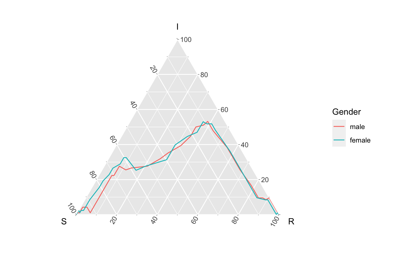
Examples

library(ggplot2)
library(dplyr)
library(ggtern); EpiCompare:::update_approved_layers()
#                ^ this generally need not be done


# geom_aggregate
EpiCompare::hagelloch_raw %>% filter(SEX %in% c("male", "female")) %>%
  ggplot(., aes(y = tI, z = tR, color = SEX)) +
  geom_aggregate() + coord_tern() +
  labs(x = "S", y = "I", z = "R",
       color = "Gender")
#> Coordinate system already present. Adding new coordinate system, which will replace the existing one.


# stat_aggregate
EpiCompare::hagelloch_raw %>% filter(SEX %in% c("male", "female")) %>%
  ggplot(., aes(y = tI, z = tR, color = SEX)) +
  geom_path(stat = StatSirAggregate) + coord_tern() +
  labs(x = "S", y = "I", z = "R",
       color = "Gender")
#> Coordinate system already present. Adding new coordinate system, which will replace the existing one.

EpiCompare::hagelloch_raw %>% dplyr::filter(SEX %in% c("male", "female")) %>%
  ggplot(., aes(y = tI, z = tR, color = SEX)) +
  stat_aggregate(geom = "path") +
  # note geom = "path" is the default
  coord_tern() +
  labs(x = "S", y = "I", z = "R",
       color = "Gender")
#> Coordinate system already present. Adding new coordinate system, which will replace the existing one.