The goal of EpiCompare is to provide the epidemiology community with easy-to-use tools to encourage comparing and assessing epidemics and epidemiology models in a time-free manner. All tools attempt to adhere to tidyverse/ggplot2 style to enhance ease of use.
Additionally, EpiCompare provides tools for time invariant analysis. This allows for ‘fairer’ comparison of epidemics and model based simulations by avoiding different scaling and shifting of time that can confound time-based comparisons.
To achieve these goals, the package contains:
-
Visualization tools to visualize SIR epidemics and simulations from SIR models in a time-free manner using
ggtern’s ternary plots and prediction bands. For agent-based SIR models we also provide visualization tools to let the user easily explore how different characteristics of the agents relate to different experiences in the epidemic. - General comparison tools to compare epidemics and epidemic models that have higher numbers of states (again in a time-free manner), allowing for the user to examine the differences between models through simulations, and if an epidemic is similar to a model through simulations and prediction bands.
-
Conversion tools to:
- Convert and then compare models from standard epidemic packages like
EpiModels,pomp, as well as internal agent-based models, and epidemics in a common framework. - Convert agent-based information into aggregate to compare in the aggregate framework described above.
- Convert and then compare models from standard epidemic packages like
Installation
You can install the developmental version of EpiCompare from github using:
# install.packages("devtools")
devtools::install_github("skgallagher/EpiCompare")
Data
Description of data including in this package can be found in the data section of the reference page of the documentation website.
Example
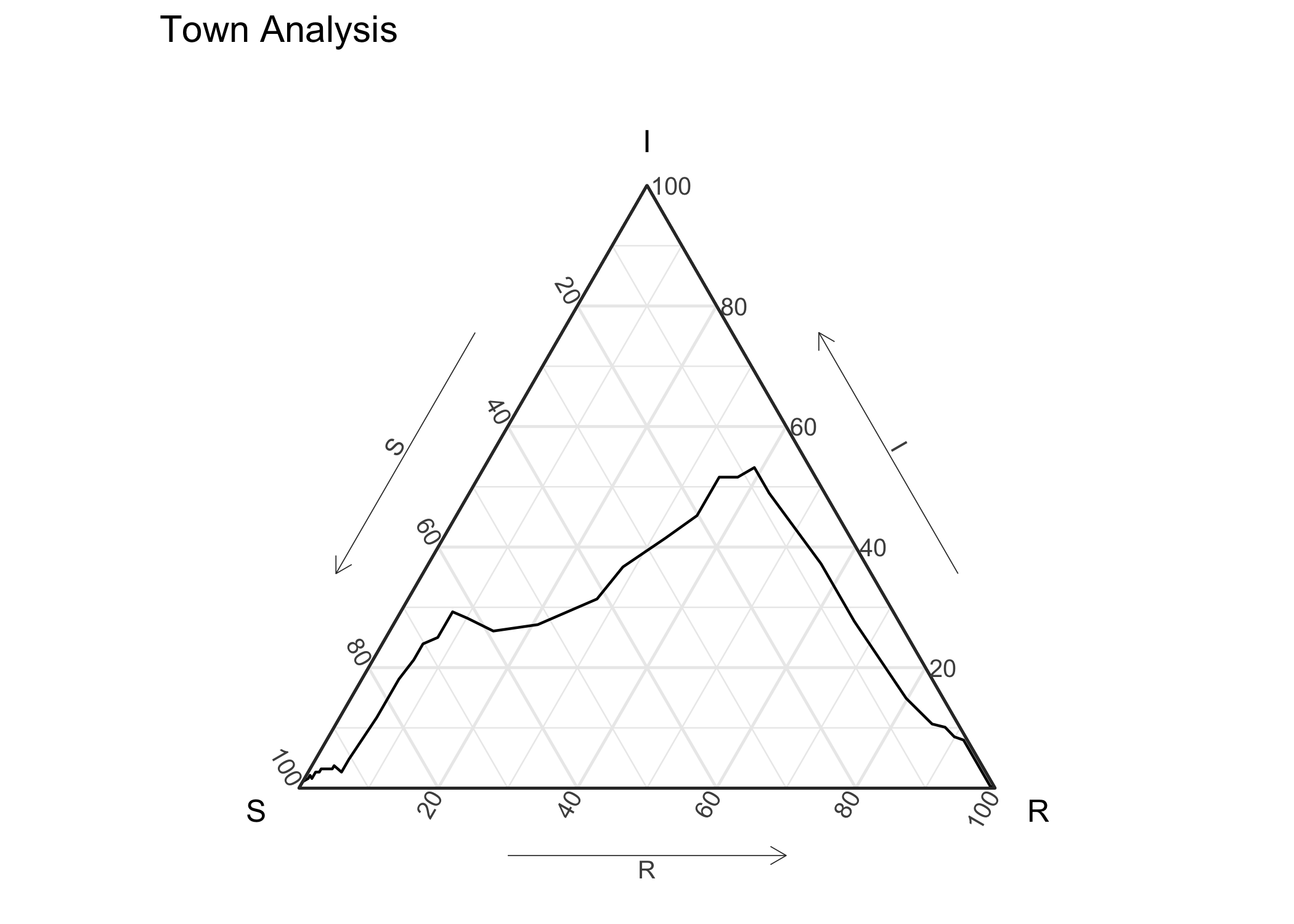
The following example comes from a Measles outbreak in Hagelloch, Germany in 1861. We have data on each child (agent) in the town.
hagelloch_raw %>%
  ggplot(aes(y = tI, z = tR)) +
    geom_aggregate() +
    coord_tern() +
    labs(x = "S", y = "I", z = "R", title = "Town Analysis") +
    theme_sir()
#> Coordinate system already present. Adding new coordinate system, which will replace the existing one.
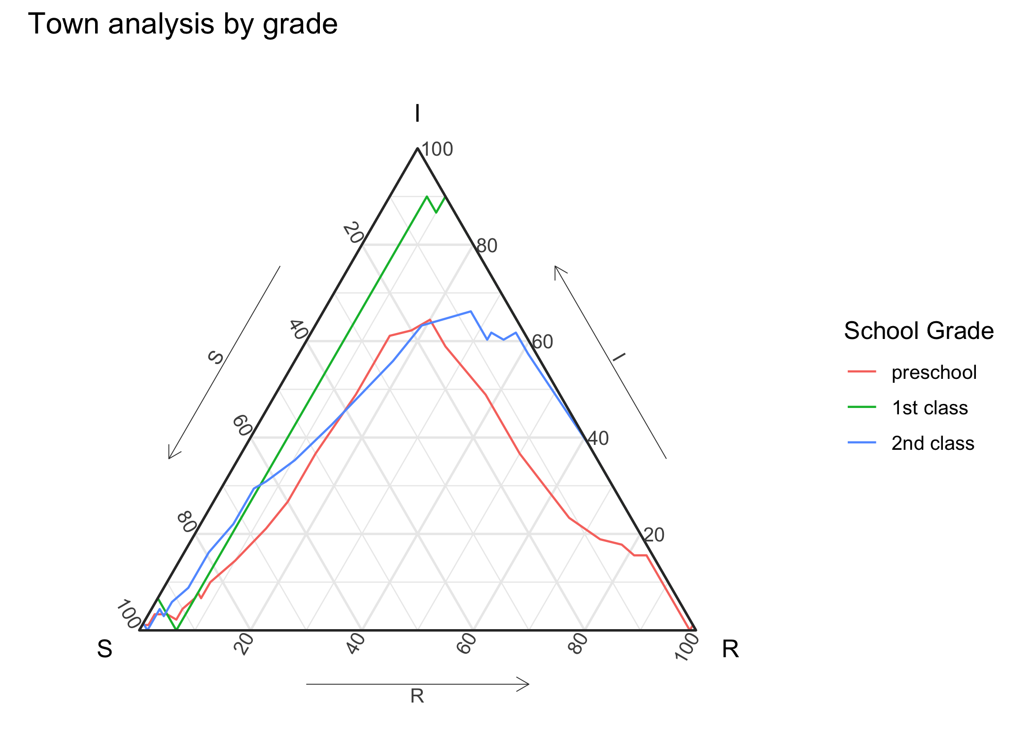
Previous work has suggested that the class (CL) the student was in effected how the experienced the outbreak. The below figure shows differences in the outbreak relative to this grouping.
hagelloch_raw %>%
  rename(`school grade` = CL) %>%
  group_by(`school grade`) %>%
  summarize(`number of students` = n())
#> `summarise()` ungrouping output (override with `.groups` argument)
#> # A tibble: 3 x 2
#>   `school grade` `number of students`
#>   <fct>                         <int>
#> 1 preschool                        90
#> 2 1st class                        30
#> 3 2nd class                        68

hagelloch_raw %>%
   ggplot(aes(y = tI, z = tR, color = CL)) +
       geom_aggregate() +
       coord_tern() +
       labs(x = "S", y = "I", z = "R",
            color = "School Grade",
            title = "Town analysis by grade") +
       theme_sir()
#> Coordinate system already present. Adding new coordinate system, which will replace the existing one.
Simulate SIR data
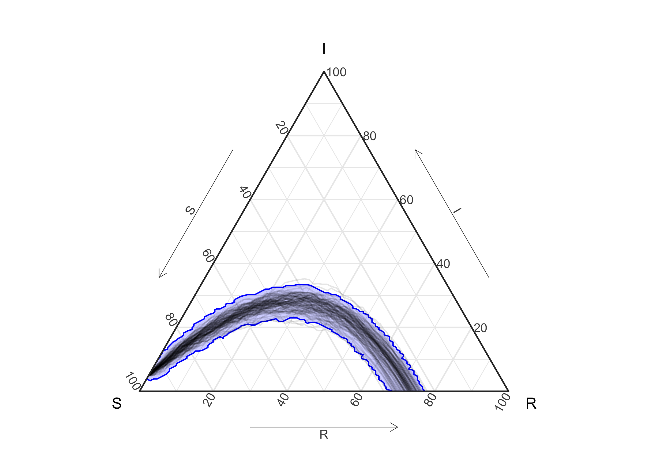
n_sims <- 100
n_time_steps <- 100
beta <- .1
gamma <- .03
init_SIR <- c(950, 50, 0)

out <- simulate_SIR_agents(n_sims = n_sims,
                           n_time_steps = n_time_steps,
                           beta = beta, gamma = gamma,
                           init_SIR = init_SIR)

df_groups <- out %>% dplyr::group_by(sim) %>%
    agents_to_aggregate(states = c(tI, tR)) %>%
    rename(S = X0, I = X1, R = X2)

df_groups %>% ggplot() +
    geom_prediction_band(aes(x = S, y = I, z = R, sim_group = as.numeric(sim)),
                         alpha = .2, fill = "blue", color = "blue") +
    geom_line(aes(x = S, y = I, z = R, group = sim), alpha = .1) +
    coord_tern() +
    theme_sir()
#> Warning: Ignoring unknown aesthetics: z
#> Coordinate system already present. Adding new coordinate system, which will replace the existing one.
#> Due to dist_params$dist_approach = "equa_dist", this may take a little while - see `filament_compression` examples for a work-around if you're making this plot multiple times
Package Creation Notes:
**We’re transferring to ~github actions~ and away from Travis CI. Thanks Travis CI for the long run (During undergrad - probably around 2015, I got introduced to Travis CI and it has been a really great tool and CIs in general are great tools). Sadly, open source packages (like ours) no longer gets infinite free resources on Travis. Dean Attali and ROpenSci have blog posts on the situation. As such, if you’re looking to learn from our mistakes from Travis, then the comments below stop making sense after December 15th, 2020.
- For writing code that works with
tidyverse1.0 vstidyverse<= 0.8.3. We followed ideas found in tidyr: in-packages, for the code, and - when working with Travis CI (using a matrix for multiple builds) - we leverage ideas in tidyverse travis on github and tidyverse principles. **This is no longer done (was removed 22 December 2020), as the rest oftidyrversehas moved on and now requirestidyr >1.0.0. - For writing your own
geoms andstats that works withggtern(which are generally restricted), the following 2 stack-exchange articles helped use do so with ease:stack-exchange: being able to access ggtern’s element right away
Finally, we’ve also leveraged ideas from R-devel: on avoiding problems with
:::inR/aaa.Rto overcome messages from CRAN relative to this hack (using:::). For some reason - when documenting forpkgdownwebsite, we need to dolibrary(ggtern); EpiCompare:::update_approved_layers()
-
geom_prediction_bandrequired not justcompute_groupbutcompute_layer- there is very little documentation on how to approach this correctly. Basically - there are problems when thecompute_groupwants to make multiplepieces/groups- and it is similar to the problem that if you do something likeaes(color = var1, group = var2)you may actually want to doaes(color = var1, group = paste(var1, var2)), if there are the samevar2values across differentvar1value, but should not necessarily be grouped together. - Now that
Rhas come out with version >= 4.0.0, we now need to call.S3method("method", "class")to define the connection forS3methods (e.g.method.classfunction), which we have for thecontainedfunction. -
Do two wrongs make a right? As of 9/23
ggternhad an issue that it messed withggplot2’s legends when loaded (it over-wrote theprint.ggplotand other functions). We’ve over-writtenggtern’sprint.ggplotto correct this problem when not producing ternary plots (code inaaa.R). - Useful Rstudio shortcuts for
Roxygen2: (a) createRoxygen2comments template withoption+command+shift+R(b) InRoxygen2comments docontrol+shift+/to format relative to 80 char limit. -
stack overflow post on how to pass
checkforrownames<-.tidy_dist_mat. - Transferring from Travis CI to github actions. We only use a single workflow file (although we use code ideas found in: check-standard/
usethis::use_github_action_check_standard()), test-coverage/usethis::use_github_action("test-coverage"). In our.github/workflows/R-CMD-check-coverage.yamlyou’ll find a (potentially not optional) approach to preform our complex checking approach (which tries to copy the ideas in our old travis file). The github action easily creates a larger matrix that allows us to run on all standard OS, R versions and our “tidyr-current” vs “tidyr-old” split. Our approach with 1 github actionyamlfile makes us only look at 8 matrix options - it’s possible that, in the future, we’ll go back to 3 files. We currently compile ourpkgdownsite on our own computers and then push - and will continue to do so due to complications withreticulateandpythonpackages on the virtual machines in github actions. - We’ve speed up some of the interval functions with
Rcpp. The setup to use this functions was slightly complex, we drafted code usingcppFunction('...')and then needed to pipe them over to the package setting. Approaches required (1)usethis::use_rcpp(), then copying C++ code intosrc/code.cpp(needed to make sure we had// [[Rcpp::export]]above each function. For make sure the functions would be compiled and available we needed to update the package documentation with 2 roxygen tags:
Contributors
- Shannon Gallagher (
skgallagher) - Benjamin LeRoy (
benjaminleroy)